In digital astrophotography, instead of taking one long exposure, we often stack many subexposures together to get at our final exposure. This lightens the load on our guiding system and prevents satellite or plane trails from ruining whole imaging sessions while still getting the increase in the signal to noise ratio that we get from long exposures.

And another issue with long exposures is, that at some point objects get saturated, i.e. photons are not counted anymore, because the pixel has reached its maximum quantum capacity.

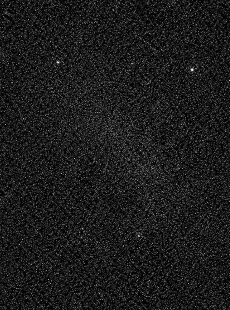
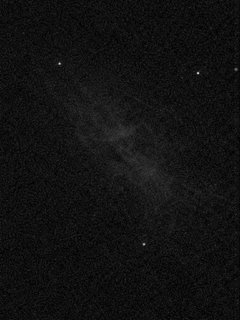
Signal to noise ratio is one of the most important factors we want to control in our astrophotography. It is so important because it allows us to bring out very dim structures that are the subject of our astrophotography. If the signal to noise ratio is low, the signal from our subject is drowned in the noise and much more difficult or even impossible to distinguish from the background noise. If the signal to noise ratio is high the subject is much more discernible from the background. Figure 1 and Figure 2 illustrate this difference visually.

The way we, as astrophotographers manipulate signal to noise ratio is by changing the exposure time of the subframes. The ideal exposure time depends not only on the target and the peculiarities of our camera but also on the light pollution we have to deal with.

Two extremes illustrate the trade-off. With perfect guiding and no satellite or plane trails, the ideal would be a single, very long exposure. Conversely, with a camera that introduced no noise, sub-exposure time would not matter: stacking many short subs would yield the same signal-to-noise ratio as one exposure of the same total duration. In practice we have neither, so we seek the shortest sub-exposure time beyond which lengthening the exposure no longer improves the signal-to-noise ratio appreciably.

In this series of articles, I will break down the theory of determining the best sub-exposure time for our frames, beginning with signal to noise ratio. In future articles, we will go into the different unwanted light sources; light polution, the moon, and twilight. And we will go deeper into signal and noise introduced by the operation of the camera and the settings we can apply to mitigate them, before putting everything together to calculate the best sub-exposure time.

Signal

To calculate the signal to noise ratio we need to have an expression for the signal that we capture and for the noise. The signal, however, does not consist wholly of the photons we receive from the nebulae, stars, and galaxies we are imaging. It also contains, unfortunately, photons that are due to light pollution and also signal due to the temperature of the sensor, the thermal signal. And we have scattered light from the Moon when it is over the horizon, or from the Sun during twilight. (We will disregard the scattered light from the Sun during daytime as no astronomical observations apart from the Sun are possible during the day.)

1. Astronomical signal ($S_*$): This is the signal we actually want to capture, the photons arriving from the celestial objects we are imaging, such as stars, nebulae, galaxies, or other deep-sky objects. This signal is typically very faint and accumulates slowly over time. The astronomical signal rate $s_a$ (i.e. the number of photons that are detected per second) depends on factors such as the brightness of the target, the aperture and focal length of the telescope, the quantum efficiency of the sensor, and atmospheric conditions.

2. Sky background signal ($S_{\mathrm{sky}}$): The sky background signal is the signal we do not want to capture. If the sky is too bright, it will be much more dificult to observe the target object. The problem is that the atmosphere scatters light from other sources increasing the brightness of the sky background. Sources are light pollution from e.g. street lights, the Moon, and the Sun (during twilight). There are also skyglow from molecular emission in the upper atmosphere, and the zodiacal light, but we will disregard their contribution as it is minimal.

   a. Light pollution signal ($S_{\mathrm{lp}}$): Light pollution refers to unwanted photons from artificial lighting sources (streetlights, city glow, etc.) that scatter in the atmosphere and enter the telescope. This is an unwanted background signal that adds to our total signal but doesn’t contribute useful information about our astronomical target. The light pollution signal rate $s_{lp}$ depends on the level of light pollution at the imaging location, the altitude of the target above the horizon, and atmospheric conditions. In heavily light-polluted areas, this can be a significant component of the total signal. There are specialised filters available that block much of the signal from light pollution, although the effectiveness depends on the light source that produces the light pollution. Narrow band filters are also very effective in blocking light pollution.

   b. Scattered Moonlight ($S_{\mathrm{moon}}$): It will be familiar to almost anyone who regularly looks up to the night sky: The sky background will be much brighter when there is a full moon, compared when the moon is below the horizon. The sky is brighter because the light from the Moon is scattered by particles in the atmosphere towards your camera sensor. This makes it very difficult to impossible to image faint objects close to the Moon, especially when it is full. Imaging, however, is possible even during full moon, when using specialised filters (often the same as used to supress light pollution), or narrow band filters.

   c. Twilight ($S_{\mathrm{twilight}}$): Sunlight is scattered in the atmosphere and makes it almost impossible to image anything other than the Sun itself during daylight. When the Sun is just below the horizon during twilight, imaging becomes possible depending on circumstances, especially when imaging with narrow band filters.

3. Thermal signal ($S_{\mathrm{T}}$): Also known as dark current, this is the signal generated by the sensor itself due to thermal energy. Even in complete darkness, electrons are thermally excited and accumulate in the sensor pixels over time. The thermal signal rate $s_T$ increases exponentially with sensor temperature, making sensor cooling (via air cooling, Peltier cooling, or liquid nitrogen) crucial for long exposures. This thermal signal can be measured and subtracted using dark frames—exposures taken with the same duration and temperature as the light frames, but with the telescope or camera lens covered. By subtracting dark frames from light frames during image processing, we can remove most of the thermal signal contribution.

The signal we capture with our sensor $S$ is thus:

\[S = S_* + S_{\mathrm{sky}} + S_{\mathrm{T}}\]

where

\[S_{\mathrm{sky}} = S_{\mathrm{lp}} + S_{\mathrm{moon}} + S_{\mathrm{twilight}}\]

The unit of $S$ is usually given as the number of electrons, i.e. $\mathrm{e}^{-}$. But that already takes quantum efficiency into account, which is a measure on how efficient the sensor is in converting photons into electrons. To avoid introducing camera specifics early, we will give the signal as the number of photons $\mathrm{\gamma}$ that are received at the sensor.

If we use $s = \frac{dS}{dt}$ to denote the signal per unit of time (in $\mathrm{\gamma}/\mathrm{s}$ or $\mathrm{\gamma}\mathrm{s}^{-1}$), we get:

\[s = \left(s_* + s_{\mathrm{sky}} + s_{\mathrm{T}}\right)\]

The value of the total signal in the image is then:

\[S = \left(s_* + s_{\mathrm{sky}} + s_{\mathrm{T}}\right) t\]

where $t$ is the exposure time.

Noise

To get to the signal to noise ratio, we, of course, also need to calculate the noise.

There are three different types of noise relevant in astrophotography:

1. Shot noise. This is the noise inherent in the signal that we receive from the sky (both from the astronomical target and the sky background). The value of shot noise is equal to the square root of the signal from the target and the sky background, $N_{\mathrm{s}} = \sqrt{S_* + S_{\mathrm{sky}}}$.
2. Thermal noise. This is the noise in the thermal signal that originates from the CCD or CMOS sensor. It is the random variation in the thermal signal. As with the shot noise, this is equal to the square root of the thermal signal, $N_{\mathrm{T}} = \sqrt{S_{\mathrm{T}}}$
3. Read noise, $N_{\mathrm{r}}$. This is the noise that is due to the electronics in the camera when reading the data from the sensor. It is only introduced when reading the camera data. It depends on the sensor and the camera electronics and the gain at which you use the camera. There is no read signal, so it does not depend on the square root of the read signal.

Poisson Distribution

Why, you may ask, are shot and thermal noise related to the signal by a square root? This is because the number of photons arriving at a sensor pixel will be different from one second to the next, without any physical change in the brightness of the source. One second, 10 photons may arrive from a small area of a source object, the next second, it may be 13 photons, and the next it may be 9, and so on. The distribution of the number of photons per second follows what we call a Poisson distribution.

The Poisson distribution is a discrete probability distribution that expresses the probability that a given number of events occurs (e.g. the arrival of photons at sensor pixel) in a fixed amount of time (e.g. a second, or the exposure time of your subframes). For a Poisson distribution, the occurrence of an event needs to be independent of the previous event, and there needs to be a mean constant rate.

This mean constant rate is the value for the pixel we are interested in, i.e what we call signal here. But the bigger the variation in the distribution the more difficult it will be with a limited exposure time to find that mean rate. The variation in this rate is what we call noise. The standard deviation of the Poisson distribution, is you may have guessed, the square root of the mean rate, i.e. what we call the signal.

Adding Noise

To add the noise contribution of the three different sources of noise, we cannot simply add them together. As a matter of fact, if these sources of noise are truly independent (and they are), we need to add them in quadrature.

\[N = \sqrt{ N_{\mathrm{s}}^2 + N_{\mathrm{T}}^2 + N_{\mathrm{r}}^2}\]

This works, because noise can be seen as vectors in probability space (as opposed to vectors in ‘normal’ Euclidean space). Each independent source of noise can be seen as a dimension in probability space. Adding them together is like adding perpendicular vectors using Pythagoras’ theorem.

Integration over time

To determine the effect of noise for each exposure we need to know how noise accumulates over time. For shot noise and thermal noise, which follow Poisson statistics, the variance accumulates linearly with time. But, as the noise in one second is independent of the noise in the previous second, we need to add them, again in quadrature.

\[N = \sqrt{n_1^2 + n_2^2 + ... + n_t^2} = \sqrt{n^2 t}\]

Where $n_1$, $n_2$ are the noise over subsequent seconds, which are, of course, equal ($n_1=n_2=n_t$) as we are talking about the variation in a distribution.

Contrary to shot and thermal noise, read noise does not accumulate over time, as it is only added when the sensor is read out, i.e. once per exposure.

So to calculate the noise over one exposure, we can calculate:

1. For shot noise: $N_s = \sqrt{n_{\mathrm{s}}^2 t} = n_{\mathrm{s}} \sqrt{t}$, where $n_{\mathrm{s}}^2 = s_* + s_{\mathrm{sky}}$ is the variance rate
2. And likewise for thermal noise: $N_{\mathrm{T}} = \sqrt{n_{\mathrm{T}}^2 t} = n_T \sqrt{t}$, where $n_{\mathrm{T}}^2 = s_{\mathrm{T}}$ is the variance rate
3. And for read noise we only have the one contribution per exposure $N_{\mathrm{r}}$

Adding these noise contributions together, we get:

\[N = \sqrt{ t \left( n_{\mathrm{s}}^2 + n_{\mathrm{T}}^2 \right)+ N_{\mathrm{r}}^2}\]

Signal to Noise Ratio

Now that we have expressions for both signal ($S$) and noise ($N$), we can derive an expression for the Signal to Noise Ratio (SNR):

\[\mathrm{SNR} = \frac{S}{N} = \frac{s t}{\sqrt{ \left( n_{\mathrm{s}}^2 + n_{\mathrm{T}}^2 \right) t + N_{\mathrm{r}}^2}}\]

where $s = s_* + s_{\mathrm{sky}} + s_{\mathrm{T}}$. Since $n_{\mathrm{s}}^2 = s = s_* + s_{\mathrm{sky}}$ and $n_{\mathrm{T}}^2 = s_{\mathrm{T}}$, we can fill this in the equation, and get:

\[\mathrm{SNR} = \frac{s t}{\sqrt{s t + N_{\mathrm{r}}^2}}\]

This is the signal to noise ratio for a single (sub-)exposure. If we stack $k$ sub-exposures together, we get the following expression for the signal to noise ratio for the stacked image:

\[\mathrm{SNR}_{\mathrm{stack}} = \frac{S k}{\sqrt{N^2 k}} = \sqrt{k} \frac{S}{N}\] \[\mathrm{SNR}_{\mathrm{stack}} = \frac{s t k}{\sqrt{s t k + N_{\mathrm{r}}^2 k}}\]

Keep in mind that the noise needs to be added in quadrature again!

Compare this with the signal to noise ratio for a single exposure with an exposure time that is the same as the accumulated exposure time of the stacked image. The total exposure time is, of course, $tk$.

\[\mathrm{SNR}_{\mathrm{long}} = \frac{s t k}{\sqrt{s t k + N_{\mathrm{r}}^2}}\]

The difference is that the read noise $N_{\mathrm{r}}$ is only added once because the sensor is only read out once, i.e. the factor $k$ is missing.

So the signal to noise ratio of the stacked image will be smaller than the signal to noise ratio of the single exposure. The ideal sub-exposure time will be the shortest exposure where

\[\text{SNR}_{\text{stack}}\approx\text{SNR}_{\text{long}}\]

while satisfying constraints from tracking, guiding, satellite tracks, and saturation.